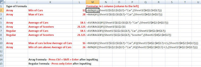
In G2 to G17 and H2 to H17 of an Excel sheet the data as shown in the picture below is recorded. Column G contains the category of vehicles sold over several months. Column H contains the corresponding count (quantity) of the category sold. (Although the data is sorted below for visual examination, it need not be sorted for the purpose of the task.). In reality the data could cover several unsorted categories (not just two as below ) spread over several months/showrooms .
The tasks are:
1. to find out minimum and maximum quantity of categories (cars ,scooters) using the entire data set.
2. to find the average of the categories
3. to find the minimum quantity of cars above the average of cars (the quantity next to the average above the average)
4. to find the maximum quantity of cars below the average of cars (the quantity next to the average below the average)
Please input the data as above in the cells in Columns G and H . Then, input the formulas as shown below in Column L (The formulas to be input are displayed in adjacent cells in Column M in the picture below.) After entering the formulas, press Ctrl + Shift + Enter if the formula type is Array (see Column J). If formula type is Regular, just press Enter. (If you did not press Ctrl + Shift + Enter while entering, press F2 in the cell and then press the Ctrl+Shift +Enter; there is no need to type the Formulas again.) If you are going to type the formulas below, instead of selecting the range of cells, please note to name the Sheet as "Sheet1"
The learning here is that Excel has ready formulas for conditional Averages (arithmetic mean) . But for more complex computation, we have to depend on Array Formulas using a combination of existing formulas.
Note: If the Array formula is entered correctly using Ctrl + Shift + Enter together, the formula will be enclosed in braces ({}) as shown in the picture below (formula shown is in L2) . The braces are not to be manually input. If not with braces, the result displayed may be incorrect.


No comments:
Post a Comment